2006 : WHAT IS YOUR DANGEROUS IDEA?

Any challenge to the normal probability bell curve can have far-reaching consequences because a great deal of modern science and engineering rests on this special bell curve. Most of the standard hypothesis tests in statistics rely on the normal bell curve either directly or indirectly. These tests permeate the social and medical sciences and underlie the poll results in the media. Related tests and assumptions underlie the decision algorithms in radar and cell phones that decide whether the incoming energy blip is a 0 or a 1. Management gurus exhort manufacturers to follow the "six sigma" creed of reducing the variance in products to only two or three defective products per million in accord with "sigmas" or standard deviations from the mean of a normal bell curve. Models for trading stock and bond derivatives assume an underlying normal bell-curve structure. Even quantum and signal-processing uncertainty principles or inequalities involve the normal bell curve as the equality condition for minimum uncertainty. Deviating even slightly from the normal bell curve can sometimes produce qualitatively different results.

The proposed dangerous idea stems from two facts about the normal bell curve.

First: The normal bell curve is not the only bell curve. There are at least as many different bell curves as there are real numbers. This simple mathematical fact poses at once a grammatical challenge to the title of Charles Murray's IQ book The Bell Curve. Murray should have used the indefinite article "A" instead of the definite article "The." This is but one of many examples that suggest that most scientists simply equate the entire infinite set of probability bell curves with the normal bell curve of textbooks. Nature need not share the same practice. Human and non-human behavior can be far more diverse than the classical normal bell curve allows.

Second: The normal bell curve is a skinny bell curve. It puts most of its probability mass in the main lobe or bell while the tails quickly taper off exponentially. So "tail events" appear rare simply as an artifact of this bell curve's mathematical structure. This limitation may be fine for approximate descriptions of "normal" behavior near the center of the distribution. But it largely rules out or marginalizes the wide range of phenomena that take place in the tails.

Again most bell curves have thick tails. Rare events are not so rare if the bell curve has thicker tails than the normal bell curve has. Telephone interrupts are more frequent. Lightning flashes are more frequent and more energetic. Stock market fluctuations or crashes are more frequent. How much more frequent they are depends on how thick the tail is — and that is always an empirical question of fact. Neither logic nor assume-the-normal-curve habit can answer the question. Instead scientists need to carry their evidentiary burden a step further and apply one of the many available statistical tests to determine and distinguish the bell-curve thickness.

One response to this call for tail-thickness sensitivity is that logic alone can decide the matter because of the so-called central limit theorem of classical probability theory. This important "central" result states that some suitably normalized sums of random terms will converge to a standard normal random variable and thus have a normal bell curve in the limit. So Gauss and a lot of other long-dead mathematicians got it right after all and thus we can continue to assume normal bell curves with impunity.

That argument fails in general for two reasons.

The first reason it fails is that the classical central limit theorem result rests on a critical assumption that need not hold and that often does not hold in practice. The theorem assumes that the random dispersion about the mean is so comparatively slight that a particular measure of this dispersion — the variance or the standard deviation — is finite or does not blow up to infinity in a mathematical sense. Most bell curves have infinite or undefined variance even though they have a finite dispersion about their center point. The error is not in the bell curves but in the two-hundred-year-old assumption that variance equals dispersion. It does not in general. Variance is a convenient but artificial and non-robust measure of dispersion. It tends to overweight "outliers" in the tail regions because the variance squares the underlying errors between the values and the mean. Such squared errors simplify the math but produce the infinite effects. These effects do not appear in the classical central limit theorem because the theorem assumes them away.

The second reason the argument fails is that the central limit theorem itself is just a special case of a more general result called the generalized central limit theorem. The generalized central limit theorem yields convergence to thick-tailed bell curves in the general case. Indeed it yields convergence to the thin-tailed normal bell curve only in the special case of finite variances. These general cases define the infinite set of the so-called stable probability distributions and their symmetric versions are bell curves. There are still other types of thick-tailed bell curves (such as the Laplace bell curves used in image processing and elsewhere) but the stable bell curves are the best known and have several nice mathematical properties. The figure below shows the normal or Gaussian bell curve superimposed over three thicker-tailed stable bell curves. The catch in working with stable bell curves is that their mathematics can be nearly intractable. So far we have closed-form solutions for only two stable bell curves (the normal or Gaussian and the very-thick-tailed Cauchy curve) and so we have to use transform and computer techniques to generate the rest. Still the exponential growth in computing power has long since made stable or thick-tailed analysis practical for many problems of science and engineering.

This last point shows how competing bell curves offer a new context for judging whether a given set of data reasonably obey a normal bell curve. One of the most popular eye-ball tests for normality is the PP or probability plot of the data. The data should almost perfectly fit a straight line if the data come from a normal probability distribution. But this seldom happens in practice. Instead real data snake all around the ideal straight line in a PP diagram. So it is easy for the user to shrug and a call any data deviation from the ideal line good enough in the absence of a direct bell-curve competitor. A fairer test is to compare the normal PP plot with the best-fitting thick-tailed or stable PP plot. The data may well line up better in a thick-tailed PP diagram than it does in the usual normal PP diagram. This test evidence would reject the normal bell-curve hypothesis in favor of the thicker-tailed alternative. Ignoring these thick-tailed alternatives favors accepting the less-accurate normal bell curve and thus leads to underestimating the occurrence of tail events.

Stable or thick-tailed probability curves continue to turn up as more scientists and engineers search for them. They tend to accurately model impulsive phenomena such as noise in telephone lines or in the atmosphere or in fluctuating economic assets. Skewed versions appear to best fit the data for the Ethernet traffic in bit packets. Here again the search is ultimately an empirical one for the best-fitting tail thickness. Similar searches will only increase as the math and software of thick-tailed bell curves work their way into textbooks on elementary probability and statistics. Much of it is already freely available on the Internet.

Thicker-tail bell curves also imply that there is not just a single form of pure white noise. Here too there are at least as many forms of white noise (or any colored noise) as there are real numbers. Whiteness just means that the noise spikes or hisses and pops are independent in time or that they do not correlate with one another. The noise spikes themselves can come from any probability distribution and in particular they can come from any stable or thick-tailed bell curve. The figure below shows the normal or Gaussian bell curve and three kindred thicker-tailed bell curves and samples of their corresponding white noise. The normal curve has the upper-bound alpha parameter of 2 while the thicker-tailed curves have lower values — tail thickness increases as the alpha parameter falls. The white noise from the thicker-tailed bell curves becomes much more impulsive as their bell narrows and their tails thicken because then more extreme events or noise spikes occur with greater frequency.

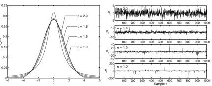
Competing bell curves: The figure on the left shows four superimposed symmetric alpha-stable bell curves with different tail thicknesses while the plots on the right show samples of their corresponding forms of white noise. The parameter describes the thickness of a stable bell curve and ranges from 0 to 2. Tails grow thicker as grows smaller. The white noise grows more impulsive as the tails grow thicker. The Gaussian or normal bell curve has the thinnest tail of the four stable curves while the Cauchy bell curve has the thickest tails and thus the most impulsive noise. Note the different magnitude scales on the vertical axes. All the bell curves have finite dispersion while only the Gaussian or normal bell curve has a finite variance or finite standard deviation.

My colleagues and I have recently shown that most mathematical models of spiking neurons in the retina can not only benefit from small amounts of added noise by increasing their Shannon bit count but they still continue to benefit from added thick-tailed or "infinite-variance" noise. The same result holds experimentally for a carbon nanotube transistor that detects signals in the presence of added electrical noise.

Thick-tailed bell curves further call into question what counts as a statistical "outlier" or bad data: Is a tail datum error or pattern? The line between extreme and non-extreme data is not just fuzzy but depends crucially on the underlying tail thickness.

The usual rule of thumb is that the data is suspect if it lies outside three or even two standard deviations from the mean. Such rules of thumb reflect both the tacit assumption that dispersion equals variance and the classical central-limit effect that large data sets are not just approximately bell curves but approximately thin-tailed normal bell curves. An empirical test of the tails may well justify the latter thin-tailed assumption in many cases. But the mere assertion of the normal bell curve does not. So "rare" events may not be so rare after all.